Introduction

In the third and final part of this series on linear models, we’ll be talking about linear mixed effect models (LMEMs). Part 1 was on simple linear models and Part 2 was on ANOVAs. LMEMs are a powerful tool for many reasons, not all of which we can get into in a single blog post. The internet has ample information about the different aspects of LMEMs and I highly recommend reading more about them if you think they will be useful for your specific data set. For this post we’ll be focusing on their benefit regarding power, how to correct our previous baseline issue, and accounting for variance across and within participants.

TAKE AWAY POINTS FROM THIS POST

• LMEMs are a way to include random variance (such as participants) without losing power.
• Contrast coding allows you to get ANOVA style results with no baseline effects.
• Random slopes can be used to account for variance from within-participant variables.

Model #1: LMEM with a random effect for participant

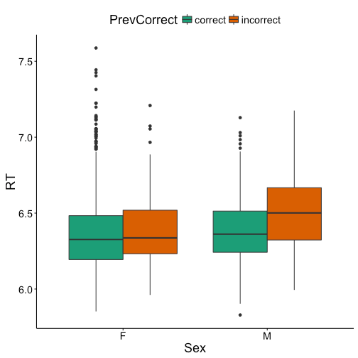
Once again we’ll be using the same data as in the previous two posts. As a reminder, this is reaction times log transformed for a lexical decision experiment. Previously we looked at the effect of previous response (correct, incorrect) and sex of participant (female, male) on response times in a simple linear model, and then in an ANOVA, including previous response as a within-participant variable. The packages for this post include languageR (for the data), ggplot2 (for plotting), and dplyr (for data manipulation). As always, we’ll start by replotting the figure of our interaction, since you should always plot your data before analyzing it.

library(languageR)
library(ggplot2)
library(dplyr)

To build an LMEM we’ll be using the ‘lmer’ (for Linear Mixed Effects Regression) call from the lme4 package. The mixed aspect of the model is the fact that we can have two types of effects: 1) fixed, and 2) random. Fixed effects are your experimental variables that you are specifically interested in testing. This is the same as what is typically coded as an independent variable in a simple linear model or an ANOVA. For this analysis our fixed effects are previous response and sex. Random effects are variables that we don’t have specific predictions about other than that they have variance that can affect how we interpret our fixed effects. This is the same thing as an error term in an ANOVA. In our ANOVA we computed average values for each participant and then included participant as an error term. Here we’ll do the same thing, only with no need to average, by including participant as a random effect. Not having to average participants’ responses is one way that LMEMs give you more power.

Below is the code for our first LMEM. The first half of the syntax is the same as our simple linear model and our ANOVA. To account for the variance by specific participants though we add ‘+ (1|Subject)’, this is the random effect of participant. This accounts for variance across different participants.

library(lme4)
lexdec_prevcorXsex.lmer = lmer(RT ~ PrevCorrect * Sex +
                              (1|Subject), REML = F, data = lexdec)
coef(summary(lexdec_prevcorXsex.lmer))

##                             Estimate Std. Error     t value
## (Intercept)               6.37413495 0.04024952 158.3654726
## PrevCorrectincorrect      0.03697533 0.02319175   1.5943309
## SexM                      0.02315971 0.06972579   0.3321541
## PrevCorrectincorrect:SexM 0.02364923 0.03915262   0.6040269

P-values are a little tricky to interpret in linear mixed effects model (and something to be left for another day), but the t-value can serve as a rough initial guide, t-values with an absolute value of 2 or above are likely significant at a threshold of p < 0.05.

Based on these results then, it looks like neither of our main effects are significant nor is our interaction. However, just as linear models had the issue of a baseline when an interaction is present, so do linear mixed effects models, they are still linear models so the same issue applies. Also like linear models we can use ‘relevel’ to change our baseline. Below is our same model but changing the baseline of previous correct to “incorrect” and sex to “M”.

lexdec_prevcorXsex_relevel.lmer = lmer(RT ~ relevel(PrevCorrect, "incorrect") * relevel(Sex, "M") +
                                      (1|Subject), REML = F, data = lexdec)
coef(summary(lexdec_prevcorXsex_relevel.lmer))

##                                                                Estimate
## (Intercept)                                                  6.45791922
## relevel(PrevCorrect, "incorrect")correct                    -0.06062456
## relevel(Sex, "M")F                                          -0.04680894
## relevel(PrevCorrect, "incorrect")correct:relevel(Sex, "M")F  0.02364923
##                                                             Std. Error
## (Intercept)                                                 0.06386223
## relevel(PrevCorrect, "incorrect")correct                    0.03154473
## relevel(Sex, "M")F                                          0.07851920
## relevel(PrevCorrect, "incorrect")correct:relevel(Sex, "M")F 0.03915262
##                                                                 t value
## (Intercept)                                                 101.1226708
## relevel(PrevCorrect, "incorrect")correct                     -1.9218600
## relevel(Sex, "M")F                                           -0.5961464
## relevel(PrevCorrect, "incorrect")correct:relevel(Sex, "M")F   0.6040269

All of our effects continue to not be significant, but the absolute value of the t-value for previous response is closer to 2 (1.92) than in the initial coding (1.59).

Model #2: LMEM with (ANOVA style) contrast coding

Similar to how we were able to get around our baseline effect with an ANOVA, we can also get rid of baselines in LMEMs via contrast coding. I won’t go into the specific details of how to do this, but if you’re interested in having ANOVA like coding for an LMEM look for a tutorial on contrast coding. The result below is a model like our ANOVA, with no baselines, but instead of taking means for each participant, we get to continue to use all of their responses.

lexdec_prevcorXsex_contrast.lmer = lmer(RT ~ PrevCorrectContrast * SexContrast +
                                        (1|Subject), data = lexdec_contrast)
coef(summary(lexdec_prevcorXsex_contrast.lmer))

##                                   Estimate Std. Error     t value
## (Intercept)                     6.41008540 0.03755813 170.6710332
## PrevCorrectContrast             0.04872980 0.01959005   2.4874772
## SexContrast                     0.03491053 0.07511627   0.4647533
## PrevCorrectContrast:SexContrast 0.02347427 0.03918010   0.5991377

Now our previous response variable is likely significant (t-value of 2.49), but our other effects continue to not be significant.

Model #3: LMEM with a random slope

The final thing we have yet to take into account that our ANOVA controlled for was the within-participant effect of previous response. In an LMEM we can account for this by updating our random effects structure. Currently participant is included only as a random intercept ‘(1|Subject)’, what we want is a random slope by previous response, which is coded as ‘(1+PrevCorrect|Subject)’. With this code the model now accounts for both the general variance across participants (the random intercept) and the variance within a given participant by previous response (the random slope). This is the same as in our ANOVA when we updated our error term of participant to include previous response to be a within-participant variable. Note, in the code below the variable in the slope is ‘PrevCorrectContrast’ since we previously contrast coded ‘PrevCorrect’.

lexdec_prevcorXsex_contrast_slope.lmer = lmer(RT ~ PrevCorrectContrast * SexContrast +
                                             (1+PrevCorrectContrast|Subject), REML = F, data = lexdec_contrast)
coef(summary(lexdec_prevcorXsex_contrast_slope.lmer))

##                                   Estimate Std. Error     t value
## (Intercept)                     6.41021327 0.03567914 179.6627911
## PrevCorrectContrast             0.04898205 0.01956688   2.5033135
## SexContrast                     0.03525743 0.07135827   0.4940903
## PrevCorrectContrast:SexContrast 0.02416548 0.03913377   0.6175096

Before getting into the results of the model I want to address one potential concern with this random effects structure. Recall that in the post on ANOVAs we confirmed that previous response really was a within-participant variable by running an ‘xtabs’ call and double checking that every participant had a ‘1’ in each cell. The call is reproduced below.

head(xtabs(~Subject+PrevCorrect, lexdec_byparticipant))

##        PrevCorrect
## Subject correct incorrect
##      A1       1         1
##      A2       1         1
##      A3       1         1
##      C        1         1
##      D        1         1
##      I        1         1

We can do the same thing now with all of our data and see not just if every participant has a data point in each cell but how many. See below for the summary.

head(xtabs(~Subject+PrevCorrect, lexdec))

##        PrevCorrect
## Subject correct incorrect
##      A1      77         2
##      A2      74         5
##      A3      73         6
##      C       78         1
##      D       76         3
##      I       68        11

As you can see the number of data points is very unbalanced, with participants having far more “correct” previous responses than “incorrect”. Our ANOVA did not take this into account. One reason why LMEMs are useful is because they can handle unbalanced data sets, however given how few data points some participants have for “incorrect”, we may not want to include previous response as a random slope. We’ll continue with it for the sake of the example, but be sure to always check the make-up of your data before building your model.

Returning to the results of the model, the effect of adding the random slope on the model is minimal, as our effect of previous response continues to be significant (t = 2.50) and our other effects continue to not be significant.

Linear Models Summary

To summarize this three part series on linear models let’s look at the final models we ran in each post. Again, as a reminder here are the full posts for Part 1 on simple linear models and Part 2 on ANOVAs.

coef(summary(lexdec_prevcorXsex.lm))

##                             Estimate  Std. Error    t value  Pr(>|t|)
## (Intercept)               6.37471510 0.007481453 852.069124 0.0000000
## PrevCorrectincorrect      0.02818559 0.029120718   0.967888 0.3332417
## SexM                      0.01679381 0.013021747   1.289674 0.1973441
## PrevCorrectincorrect:SexM 0.10515531 0.047704121   2.204323 0.0276388

summary(lexdec_prevcorXsex_byparticipant.aov)

## 
## Error: Subject
##           Df Sum Sq Mean Sq F value Pr(>F)
## Sex        1 0.0355 0.03547   0.567  0.461
## Residuals 19 1.1882 0.06254               
## 
## Error: Subject:PrevCorrect
##                 Df  Sum Sq Mean Sq F value Pr(>F)  
## PrevCorrect      1 0.04701 0.04701   5.569 0.0291 *
## PrevCorrect:Sex  1 0.01364 0.01364   1.615 0.2191  
## Residuals       19 0.16039 0.00844                 
## ---
## Signif. codes:  0 '***' 0.001 '**' 0.01 '*' 0.05 '.' 0.1 ' ' 1

coef(summary(lexdec_prevcorXsex_contrast_slope.lmer))

##                                   Estimate Std. Error     t value
## (Intercept)                     6.41021327 0.03567914 179.6627911
## PrevCorrectContrast             0.04898205 0.01956688   2.5033135
## SexContrast                     0.03525743 0.07135827   0.4940903
## PrevCorrectContrast:SexContrast 0.02416548 0.03913377   0.6175096

Overall we see that the ANOVA and LMEM are pretty similar, showing a significant effect only for previous response, while the initial simple linear model included a significant interaction of previous response and sex. From this we can conclude that incorporating participant specific variance in the model is important to understand which effects are real. The lack of a significant interaction in our LMEM showed us that the disappearance of the effect in the ANOVA was not simple due to a lack of power.

Conclusion

I hope you enjoyed this three part series on linear models. We only briefly went over linear mixed effects models, but they are a very powerful tool for inferential statistics and have been fully adopted by several disciplines. In addition to allowing you to use all data points, instead of averaging and losing power, they also can handle a more complex random effects structure (for example, including both participant and item as a random effect) and can be used when you have a binary dependent variable (for example, correct versus incorrect). If you’re interested in learning more about linear mixed effects models stay tuned for a lesson in my new R course “R for Publication”.