Introduction

In the last post we looked at linear regressions and particularly what happens when you add an interaction to a linear regression. We found that baselines make it difficult to interpret main effects, and confirmed that plotting data is the best way to really understand what’s going on. Today we’ll look at the same data as last time, but use a statistic that gets rid of our baseline issue for interpreting main effects.

TAKE AWAY POINTS FROM THIS POST

• ANOVAs can be used to look at main effects when an interaction is in the model.
• When running an ANOVA with multiple measurements for each participant it is standard practice to get means for each participant first.
• ANOVAs can take into account within-participant variables.

Model #1: ANOVA with two variables and an interaction

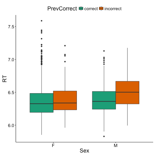
To start we’ll use the same data as in the previous post, but now running an analysis of variance (ANOVA) instead of a simple linear model. As a reminder, this is reaction times log transformed for a lexical decision experiment. Previously we looked at the effect of previous response (correct, incorrect) and sex of participant (female, male) on response times. In addition to using the languageR and ggplot2 packages, I’ll also be using dplyr for some data manipulation and gridExtra for figure displaying. We’ll start by replotting the figure of our interaction, since you should always plot your data before analyzing it.

library(languageR)
library(ggplot2)
library(dplyr)
library(gridExtra)

To build the ANOVA we’ll use the ‘aov’ call, but other than that the syntax is the same as our previous ‘lm’ call.

lexdec_prevcorXsex.aov = aov(RT ~ PrevCorrect * Sex, data = lexdec)
summary(lexdec_prevcorXsex.aov)

##                   Df Sum Sq Mean Sq F value  Pr(>F)   
## PrevCorrect        1   0.51  0.5103   8.826 0.00301 **
## Sex                1   0.22  0.2235   3.865 0.04946 * 
## PrevCorrect:Sex    1   0.28  0.2809   4.859 0.02764 * 
## Residuals       1655  95.69  0.0578                   
## ---
## Signif. codes:  0 '***' 0.001 '**' 0.01 '*' 0.05 '.' 0.1 ' ' 1

The ANOVA above finds a significant effect of previous response, sex, and a significant interaction of previous response and sex. Recall that for the linear model we lost our significant main effects due to the interaction adding baselines for each variable. The ANOVA recenters each variable for us, such that there is no baseline for main effects. As a result, the ANOVA gives us the results of the main effects for each variable, and the interaction.

To confirm this look at our linear models again. You’ll see that the p-values for the main effects in the first model without the interaction are roughly equivalent to the p-values for the main effects in the ANOVA, and the p-value for the interaction in the second model is roughly the same as in the ANOVA. Note though that in the linear model p-values are based on t-values, while in the ANOVA they are based on F-values.

lexdec_prevcor_sex.lm = lm(RT ~ PrevCorrect + Sex, data = lexdec)
coef(summary(lexdec_prevcor_sex.lm))

##                        Estimate  Std. Error    t value    Pr(>|t|)
## (Intercept)          6.37212873 0.007397478 861.391991 0.000000000
## PrevCorrectincorrect 0.06737093 0.023092187   2.917477 0.003576318
## SexM                 0.02462915 0.012541806   1.963764 0.049724544

lexdec_prevcorXsex.lm = lm(RT ~ PrevCorrect * Sex, data = lexdec)
coef(summary(lexdec_prevcorXsex.lm))

##                             Estimate  Std. Error    t value  Pr(>|t|)
## (Intercept)               6.37471510 0.007481453 852.069124 0.0000000
## PrevCorrectincorrect      0.02818559 0.029120718   0.967888 0.3332417
## SexM                      0.01679381 0.013021747   1.289674 0.1973441
## PrevCorrectincorrect:SexM 0.10515531 0.047704121   2.204323 0.0276388

Model #2: ANOVA by participant

It looks like ANOVAs are the way to go to be able to interpret main effects and interactions. However, there is some key variability that we haven’t been accounting for. Each participant has multiple data points, and a given participant may behave differently from another participant. Right now though our model treats two data points from the same participant just like two data points from two unique participants. To account for this variability researchers often conduct an ANOVA by-participant (or by-subject) in which the mean of the dependent variable (here reaction times) is found for each participant for each variable in the analysis. The ANOVA is then run on these means, instead of the original raw data.

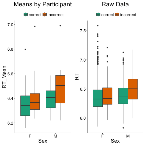
To show how this is done I’ve summarized the data with means for each participant for each level of previous response (correct, incorrect) and sex (female, male). You can see the first few rows below. Note that there are two rows for each participant, one for each level of previous response since no participant was 100% correct or incorrect. Furthermore, each participant also has only one sex assigned to them, so both rows for a given participant has the same value for sex. I’ve named this summary column ‘RT_Mean’.

head(lexdec_byparticipant)

## Source: local data frame [6 x 4]
## 
##   Subject PrevCorrect    Sex  RT_Mean
##    (fctr)      (fctr) (fctr)    (dbl)
## 1      A1     correct      F 6.273498
## 2      A1   incorrect      F 6.440793
## 3      A2     correct      M 6.220342
## 4      A2   incorrect      M 6.220954
## 5      A3     correct      F 6.394754
## 6      A3   incorrect      F 6.433998

Here’s a boxplot of what our two variables look like, now plotting the means for each participant. Comparing to the boxplot with all the raw data, you’ll notice it’s a bit different, but not dramatically so. Particularly there are fewer outliers and the effect of previous responses seems larger for both sexes.

Now we can run our same ANOVA as from before, however with far fewer data points due to the summarizing. As a result none of our effects are significant as can be seen in the output of the ANOVA. Despite the fact that the effect of the interaction looks larger in the boxplot the reduction in power (from 1659 data points to 42 data points) makes the effect go away.

lexdec_byparticipant_prevcorXsex.aov = aov(RT_Mean ~ PrevCorrect * Sex, data = lexdec_byparticipant)
summary(lexdec_byparticipant_prevcorXsex.aov)

##                 Df Sum Sq Mean Sq F value Pr(>F)
## PrevCorrect      1 0.0470 0.04701   1.325  0.257
## Sex              1 0.0355 0.03547   1.000  0.324
## PrevCorrect:Sex  1 0.0136 0.01364   0.384  0.539
## Residuals       38 1.3486 0.03549

Model #3: ANOVA with within-participant variable

Our current ANOVA is still failing to account for some variance. The ANOVA above does not control for the fact that the previous response variable is within-participant, as each participant has previous responses that are correct and incorrect. Sex is a between-participant variable since each participant is only one sex. If you are ever in doubt about whether a variable is within-participant or between-participant ‘xtabs’ is a useful call; it summarizes the number of data points you have within a given cell. If you see any 0s in the output you know it is a between-participant variable because you don’t have any data points for that cell. For example, below there are no 0s for the comparison of participant with previous response but there are for the comparison of participant with sex.

head(xtabs(~Subject+PrevCorrect, lexdec_byparticipant))

##        PrevCorrect
## Subject correct incorrect
##      A1       1         1
##      A2       1         1
##      A3       1         1
##      C        1         1
##      D        1         1
##      I        1         1

head(xtabs(~Subject+Sex, lexdec_byparticipant))

##        Sex
## Subject F M
##      A1 2 0
##      A2 0 2
##      A3 2 0
##      C  2 0
##      D  0 2
##      I  2 0

To deal with this we can add an error term of participant by previous response to our model, basically telling the ANOVA to compare the previous response levels within participant instead of across participants. We now get two types of information in the output. First are the between-participant variables, specifically sex. Similar to the first model there is no effect of sex. In the second part of the output are any analyses that include the within-participant variable, previous response. As you can see previous response is now significant in our new model, although the interaction continues to not be significant.

lexdec_byparticipant_prevcorXsex.aov = aov(RT_Mean ~ PrevCorrect * Sex + Error(Subject/PrevCorrect), data = lexdec_byparticipant)
summary(lexdec_byparticipant_prevcorXsex.aov)

## 
## Error: Subject
##           Df Sum Sq Mean Sq F value Pr(>F)
## Sex        1 0.0355 0.03547   0.567  0.461
## Residuals 19 1.1882 0.06254               
## 
## Error: Subject:PrevCorrect
##                 Df  Sum Sq Mean Sq F value Pr(>F)  
## PrevCorrect      1 0.04701 0.04701   5.569 0.0291 *
## PrevCorrect:Sex  1 0.01364 0.01364   1.615 0.2191  
## Residuals       19 0.16039 0.00844                 
## ---
## Signif. codes:  0 '***' 0.001 '**' 0.01 '*' 0.05 '.' 0.1 ' ' 1

Conclusion

Today we’ve found that ANOVAs can be a useful way to look at both main effects and interactions. We were also able to account for variance between participants and say which variables were within-participant. However, by averaging participants’ data we lost a lot of power, and some of our effects went away. Also the design was unbalanced for various reasons, including some participants having more or fewer correct or incorrect previous responses than other participants, which is lost by averaging. In Part 3 we’ll look at linear mixed effects models which can take care of these issues and more!