Welcome!
Hello and welcome to to my new blog! My goal with this blog is to talk about things that I found odd or difficult during my time as a PhD student. I won’t be going into the details of the math behind particular models, but instead focusing on how best to analyze your data set with the correct statistics and how to interpret the results you get. All analyses will be conducted in R, but many of the core principles apply to other statistical programming languages as well. Topics will range from simple aspects of classical statistics that are commonly misunderstood by researchers, to advanced models that are only recently becoming the norm in scientific papers. Comments and questions are of course welcome.
Introduction
The first topic I wanted to discuss is what happens when you add an interaction to a linear model or “Why You Should Always Plot Your Data First”. In the rush to get a p-value less than 0.05 I often found myself running analyses before actually looking at my data. This can lead to several problems including, not knowing if your data has a normal distribution, not noticing outliers, or not knowing what an interaction really means (and in turn how to interpret your main effects). This last one is what I’ll be focusing on today. This post will be the first part in a three part series on using linear models to explain your data.
TAKE AWAY FROM TODAY’S POST
- Plot your data before beginning analyses.
- When interpreting linear models with interactions, be sure to bear in mind the baselines of all of the variables in the model.
- Relevel variables to better understand interactions.
Model #1: Model with one variable
The data I’ll be analyzing come from the package languageR. The package contains several data sets from language research. The one for today’s example are from the ‘lexdec’ data set, which provides lexical decision latencies (or how long it took a person to decide if a string of characters on a screen is a word or not) for 79 English nouns. In addition to the languageR package I’ll also be using the ggplot2 package for plotting the results.
library(languageR)
library(ggplot2)
A common goal for these types of experiments is to see which factors affect how quickly a person provides their response, in this case word or non-word. To start off with we’ll see if how the participant answered the previous item (correct, incorrect) affected their speed on the current item (speed in reaction times log transformed). To do this we will build a simple linear model to see if previous response (PrevCorrect) predicts reaction times (RT).
lexdec_prevcor.lm = lm(RT ~ PrevCorrect, data = lexdec)
summary(lexdec_prevcor.lm)
##
## Call:
## lm(formula = RT ~ PrevCorrect, data = lexdec)
##
## Residuals:
##     Min      1Q  Median      3Q     Max
## -0.5513 -0.1709 -0.0399  0.1150  1.2070
##
## Coefficients:
##                      Estimate Std. Error  t value Pr(>|t|)
## (Intercept)          6.380259   0.006136 1039.836  < 2e-16 ***
## PrevCorrectincorrect 0.068503   0.023105    2.965  0.00307 **
## ---
## Signif. codes:  0 '***' 0.001 '**' 0.01 '*' 0.05 '.' 0.1 ' ' 1
##
## Residual standard error: 0.2409 on 1657 degrees of freedom
## Multiple R-squared:  0.005277,   Adjusted R-squared:  0.004677
## F-statistic: 8.791 on 1 and 1657 DF,  p-value: 0.003071
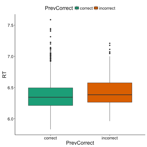
The model shows us that indeed there does appear to be an effect, such that participants are slower (longer RTs) if they got the previous item incorrect. If we plot this effect we see that the difference is there, although it seems very small.

Model #2: Model with two variables
While previous response accounted for some of variance in RTs, it’s possible that other variables are predictive as well. Next, we’ll see if sex of the participant (female, male) had any effect. For now we’ll simply add the variable to the model as another main effect, not as an interaction.
lexdec_prevcor_sex.lm = lm(RT ~ PrevCorrect + Sex, data = lexdec)
summary(lexdec_prevcor_sex.lm)
##
## Call:
## lm(formula = RT ~ PrevCorrect + Sex, data = lexdec)
##
## Residuals:
##      Min       1Q   Median       3Q      Max
## -0.56781 -0.17092 -0.04413  0.11527  1.21518
##
## Coefficients:
##                      Estimate Std. Error t value Pr(>|t|)
## (Intercept)          6.372129   0.007397 861.392  < 2e-16 ***
## PrevCorrectincorrect 0.067371   0.023092   2.917  0.00358 **
## SexM                 0.024629   0.012542   1.964  0.04972 *
## ---
## Signif. codes:  0 '***' 0.001 '**' 0.01 '*' 0.05 '.' 0.1 ' ' 1
##
## Residual standard error: 0.2407 on 1656 degrees of freedom
## Multiple R-squared:  0.007588,   Adjusted R-squared:  0.00639
## F-statistic: 6.331 on 2 and 1656 DF,  p-value: 0.001824
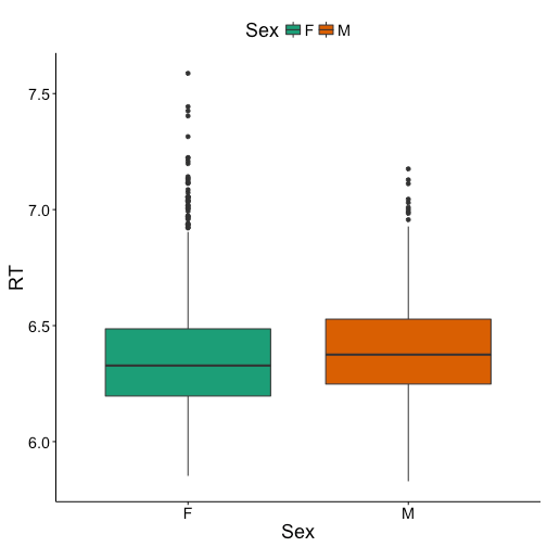
The model finds that sex also accounts for some of the variance, such that men have slower responses than women. Also, our effect of previous response still holds. If we plot the sex difference we can see that the effect is there, but like the previous response effect very small.

Model #3: Model with two variables and an interaction
Okay, we’ve now found two significant effects, but what happens if we add an interaction the model? The model below includes our two variables and the interaction of those variables.
lexdec_prevcorXsex.lm = lm(RT ~ PrevCorrect * Sex, data = lexdec)
summary(lexdec_prevcorXsex.lm)
##
## Call:
## lm(formula = RT ~ PrevCorrect * Sex, data = lexdec)
##
## Residuals:
##      Min       1Q   Median       3Q      Max
## -0.56256 -0.17092 -0.04144  0.11589  1.21260
##
## Coefficients:
##                           Estimate Std. Error t value Pr(>|t|)
## (Intercept)               6.374715   0.007481 852.069   <2e-16 ***
## PrevCorrectincorrect      0.028186   0.029121   0.968   0.3332
## SexM                      0.016794   0.013022   1.290   0.1973
## PrevCorrectincorrect:SexM 0.105155   0.047704   2.204   0.0276 *
## ---
## Signif. codes:  0 '***' 0.001 '**' 0.01 '*' 0.05 '.' 0.1 ' ' 1
##
## Residual standard error: 0.2405 on 1655 degrees of freedom
## Multiple R-squared:  0.01049,    Adjusted R-squared:  0.0087
## F-statistic:  5.85 on 3 and 1655 DF,  p-value: 0.0005674
As you can see there is a significant interaction, but we’ve also lost the significant effects for the individual variables. And now we’ve come to the pitfall that many have come to before. The reason for the apparent disappearance of our effect is because the results for the variables themselves are no longer based on the entire data set, but instead based on a subset of the data set dictated by the other variable. R by default codes variables’ baselines alphabetically, in this case for PrevCorrect the baseline is “correct” and for Sex it is “F”. So, the effect of PrevCorrect in the model is only in reference to the data from females, since “F”“ is the baseline for Sex. All this model is telling us is that there is no effect of previous response for females, not for the data set overall.
To better demonstrate this we can relevel the baseline level for a variable. Below I’ve releveled Sex to have “M” as the baseline. As you can see PrevCorrect is significant again, showing that previous response is a significant predictor for data from male participants.
lexdec_prevcorXsex_resex.lm = lm(RT ~ PrevCorrect * relevel(Sex, "M"), data = lexdec)
summary(lexdec_prevcorXsex_resex.lm)
##
## Call:
## lm(formula = RT ~ PrevCorrect * relevel(Sex, "M"), data = lexdec)
##
## Residuals:
##      Min       1Q   Median       3Q      Max
## -0.56256 -0.17092 -0.04144  0.11589  1.21260
##
## Coefficients:
##                                         Estimate Std. Error t value
## (Intercept)                              6.39151    0.01066 599.689
## PrevCorrectincorrect                     0.13334    0.03778   3.529
## relevel(Sex, "M")F                      -0.01679    0.01302  -1.290
## PrevCorrectincorrect:relevel(Sex, "M")F -0.10516    0.04770  -2.204
##                                         Pr(>|t|)
## (Intercept)                              < 2e-16 ***
## PrevCorrectincorrect                    0.000429 ***
## relevel(Sex, "M")F                      0.197344
## PrevCorrectincorrect:relevel(Sex, "M")F 0.027639 *
## ---
## Signif. codes:  0 '***' 0.001 '**' 0.01 '*' 0.05 '.' 0.1 ' ' 1
##
## Residual standard error: 0.2405 on 1655 degrees of freedom
## Multiple R-squared:  0.01049,    Adjusted R-squared:  0.0087
## F-statistic:  5.85 on 3 and 1655 DF,  p-value: 0.0005674
The same applies to the sudden lack of an effect of sex. The model with the interaction tells us that there is no effect of sex when the baseline for PrevCorrect is “correct”. However, if we relevel PrevCorrect to “incorrect” we see that the sex effect returns.
lexdec_prevcorXsex_reprevcor.lm = lm(RT ~ relevel(PrevCorrect, "incorrect") * Sex, data = lexdec)
summary(lexdec_prevcorXsex_reprevcor.lm)
##
## Call:
## lm(formula = RT ~ relevel(PrevCorrect, "incorrect") * Sex, data = lexdec)
##
## Residuals:
##      Min       1Q   Median       3Q      Max
## -0.56256 -0.17092 -0.04144  0.11589  1.21260
##
## Coefficients:
##                                               Estimate Std. Error t value
## (Intercept)                                    6.40290    0.02814 227.511
## relevel(PrevCorrect, "incorrect")correct      -0.02819    0.02912  -0.968
## SexM                                           0.12195    0.04589   2.657
## relevel(PrevCorrect, "incorrect")correct:SexM -0.10516    0.04770  -2.204
##                                               Pr(>|t|)
## (Intercept)                                    < 2e-16 ***
## relevel(PrevCorrect, "incorrect")correct       0.33324
## SexM                                           0.00795 **
## relevel(PrevCorrect, "incorrect")correct:SexM  0.02764 *
## ---
## Signif. codes:  0 '***' 0.001 '**' 0.01 '*' 0.05 '.' 0.1 ' ' 1
##
## Residual standard error: 0.2405 on 1655 degrees of freedom
## Multiple R-squared:  0.01049,    Adjusted R-squared:  0.0087
## F-statistic:  5.85 on 3 and 1655 DF,  p-value: 0.0005674
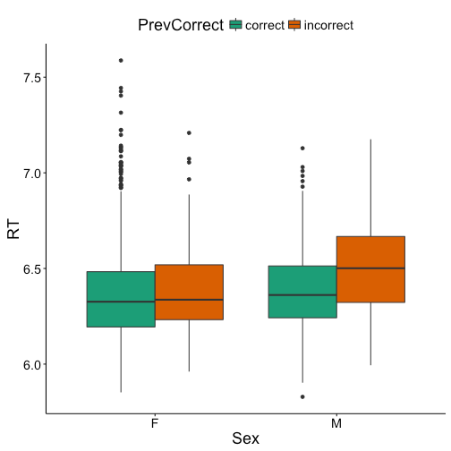
What does all of this mean in the end? Well the first two models showed us that there is a main effect of both previous response and sex in the data set. However, in the model with the interaction, where the summary statistics of PrevCorrect and Sex are only on subsets of the data, we found out that the effect of previous response was limited to males, and the sex effect was limited to items where the previous response was incorrect, thus the significant interaction.
An even easier way to see this all from the beginning would have been to plot the interaction as done below, where the effects (and lack there of) are visually apparent. As expected females do not show the effect of previous response but males do, and females only differ from males when the previous response was incorrect.

Conclusion
In summary, be sure to always plot your data before running analyses to be sure you understand what’s going on. When running a linear model with interactions be aware of the baselines for variables. In Part 2 we’ll explore a different statistical test that let’s us see main effects and interactions in the same model, Analysis of Variance aka ANOVA.
2 Pingbacks